Simulating March Madness in R
When my brother told me that his family trip to Vegas just so happened to coincide with the commencement of March Madness, I laughed. Then he asked me to do my data science thing for his bracket selection and I sighed… and said that I’d give it a shot.
I don’t get into college sports. My alma mater, UIC, is more of a research powerhouse than a sports powerhouse. And my feeling is that I’d rather pay to see professionals than pay to see college students work for free. Although, my neighbor and ex-classmate, Curtis Granderson, did donate a ton of money so that the baseball team could build a new stadium. Every year I intend on becoming a regular attendee, but with an Opening Day in February, I lack the dedication.
FiveThirtyEight
Where does a data scientist start? With data! Of course FiveThirtyEight.com has a great data set. I was able to get a head start using their 2017 data. If you go to the bottom you can see that they let you download the csv file. Like true professionals, their csv format is almost identical this year. This made updating my code very easy… And now on to the coding for all the nerds out there.
If you’re here for the insights, spoiler alert: There ain’t much difference between my results and 538’s except that Villanova is going all the way baby!
Simulating the tournament
First I downloaded the data from the website and saved it. I could’ve used the download.file() function to highlight my sweet data science skills, but I don’t need your validation hipster data scientists! The second and third lines of code aren’t necessary right now, but if you look at the 2017 data, they eventually added the women’s bracket and appended forecasts from later dates in the tournament. If you look at this code after today, March 13th, you might want to use this.
Here’s what the data looks like:
dat <- read.csv("fivethirtyeight_ncaa_forecasts_2018.csv", stringsAsFactors = FALSE)
dat <- dat[which(dat$gender == "mens" &
                     dat$forecast_date == "2018-03-12"), ]
dat18 <- dat
dat18[, 5:10] <- dat[, 5:10] / dat[, 4:9]
head(dat18)

##   gender forecast_date playin_flag rd1_win   rd2_win   rd3_win   rd4_win
## 1   mens    2018-03-12           0       1 0.9826613 0.8756271 0.7719774
## 2   mens    2018-03-12           0       1 0.9853076 0.8759937 0.7739714
## 3   mens    2018-03-12           0       1 0.9580615 0.8417617 0.5785810
## 4   mens    2018-03-12           0       1 0.9541362 0.8007723 0.8081242
## 5   mens    2018-03-12           0       1 0.9227570 0.8134675 0.5388669
## 6   mens    2018-03-12           0       1 0.9326323 0.8311586 0.6775802
##     rd5_win   rd6_win   rd7_win team_alive team_id      team_name
## 1 0.7113416 0.6808053 0.5592682          1     258       Virginia
## 2 0.7441768 0.5854901 0.5964982          1     222      Villanova
## 3 0.6178763 0.5637075 0.5951155          1     150           Duke
## 4 0.5157563 0.4794573 0.5201710          1    2305         Kansas
## 5 0.6040952 0.4937998 0.5330441          1     127 Michigan State
## 6 0.4376696 0.5804383 0.4625857          1    2132     Cincinnati
##   team_rating team_region team_seed
## 1       94.31       South         1
## 2       94.92        East         1
## 3       92.59     Midwest         2
## 4       90.88     Midwest         1
## 5       91.67     Midwest         3
## 6       91.06       South         2
From here we simulate tournament play.
I handled the First Four awkwardness last year using code like this. mat.17 is so named because at that point there are 17 teams in the region. The resulting mat.16 brings us to the more standard 16-team tournament.
mat.17 <- dat18[which(dat18$team_region == "Midwest" &
                          dat18$gender == "mens" &
                          dat18$forecast_date == "2018-03-12"),]

first.four <- which(mat.17$team_seed == "11a" | mat.17$team_seed == "11b")
mat.16 <- rbind(mat.17[-first.four, ],
                mat.17[sample(x = first.four, size = 1,
                              prob = mat.17[first.four, "rd1_win"]), ])
mat.16[16, "team_seed"] <- "11"
mat.16[, "team_seed"] <- as.numeric(mat.16[, "team_seed"])
mat.16 <- mat.16[order(mat.16$team_seed), ]
mat.16

##    gender forecast_date playin_flag   rd1_win    rd2_win   rd3_win
## 4    mens    2018-03-12           0 1.0000000 0.95413624 0.8007723
## 3    mens    2018-03-12           0 1.0000000 0.95806152 0.8417617
## 5    mens    2018-03-12           0 1.0000000 0.92275700 0.8134675
## 23   mens    2018-03-12           0 1.0000000 0.79816102 0.5216653
## 25   mens    2018-03-12           0 1.0000000 0.61981004 0.5658178
## 21   mens    2018-03-12           0 1.0000000 0.57353779 0.2372587
## 34   mens    2018-03-12           0 1.0000000 0.58044746 0.1972652
## 22   mens    2018-03-12           0 1.0000000 0.63156066 0.2501076
## 42   mens    2018-03-12           0 1.0000000 0.36843934 0.1838281
## 36   mens    2018-03-12           0 1.0000000 0.41955254 0.1628328
## 43   mens    2018-03-12           1 0.5877584 0.46073568 0.2195347
## 46   mens    2018-03-12           0 1.0000000 0.38018996 0.4731856
## 56   mens    2018-03-12           0 1.0000000 0.20183898 0.2627198
## 53   mens    2018-03-12           0 1.0000000 0.07724300 0.3434272
## 61   mens    2018-03-12           0 1.0000000 0.04193848 0.2556496
## 57   mens    2018-03-12           0 1.0000000 0.04586376 0.2238489
##      rd4_win   rd5_win   rd6_win   rd7_win team_alive team_id
## 4  0.8081242 0.5157563 0.4794573 0.5201710          1    2305
## 3  0.5785810 0.6178763 0.5637075 0.5951155          1     150
## 5  0.5388669 0.6040952 0.4937998 0.5330441          1     127
## 23 0.2713751 0.2677178 0.3011693 0.3526738          1       2
## 25 0.2799675 0.2758782 0.3023590 0.3538549          1     228
## 21 0.3506738 0.4321323 0.4005194 0.4480226          1    2628
## 34 0.2760591 0.3406308 0.2712332 0.3225783          1     227
## 22 0.6034425 0.2983157 0.3133056 0.3646722          1    2550
## 42 0.5025144 0.2280794 0.2512151 0.3020226          1     152
## 36 0.2996991 0.3644445 0.3087235 0.3601552          1     201
## 43 0.2710992 0.3507883 0.2756146 0.3270297          1     183
## 46 0.1810895 0.1809292 0.2254796 0.2750365          1     166
## 56 0.1242912 0.1252019 0.1478387 0.1891547          1     232
## 53 0.1640383 0.2287034 0.1766618 0.2218949          1    2083
## 61 0.1059174 0.1482783 0.1137260 0.1489058          1     314
## 57 0.2781671 0.1104513 0.1245251 0.1618349          1     219
##                team_name team_rating team_region team_seed
## 4                 Kansas       90.88     Midwest         1
## 3                   Duke       92.59     Midwest         2
## 5         Michigan State       91.67     Midwest         3
## 23                Auburn       84.04     Midwest         4
## 25               Clemson       84.15     Midwest         5
## 21       Texas Christian       84.84     Midwest         6
## 34          Rhode Island       83.07     Midwest         7
## 22            Seton Hall       85.05     Midwest         8
## 42  North Carolina State       81.74     Midwest         9
## 36              Oklahoma       82.10     Midwest        10
## 43              Syracuse       81.86     Midwest        11
## 46      New Mexico State       79.79     Midwest        12
## 56 College of Charleston       76.44     Midwest        13
## 53              Bucknell       78.25     Midwest        14
## 61                  Iona       74.79     Midwest        15
## 57          Pennsylvania       75.55     Midwest        16
Next I created a general tournament function using my knowledge of tournaments gained from 10 years of wrestling; i.e. the best team plays the worst team, the second best team plays the second worst team, etc. So if you order the data frames as we’ve done above, this makes picking the teams being simulated very easy. That is expressed in the ind <- c(i, nrow(mat.big) + 1 - i) line of code. The line of code after that simulates a game by pulling one sample (or team) according to their win probability in a given round as prescribed by 538. Lastly, we collect our winners and output them as mat.small.
Tournament.Round <- function(mat.big = mat.16, rd = "rd2_win"){
  vec.small <- c()
  for(i in 1:(nrow(mat.big) / 2)){
    ind <- c(i, nrow(mat.big) + 1 - i)
    temp <- sample(x = ind, size = 1, prob = mat.big[ind, rd])
    vec.small <- c(vec.small, temp)
  }
  mat.small <- mat.big[vec.small, ]
}
Now we use that Tournament.Round() function and the earlier First Four code to create a function that will simulate an entire 17-team regional outcome. The First Four code is kind of awkward and long. If I were to do this for work, I’d clean it up and make it work in perpetuity, but I don’t work for you!
Region.Simulation <- function(region = "Midwest", dat = dat18){
  mat.17 <- dat[which(dat$team_region == region &
                          dat$gender == "mens" &
                          dat$forecast_date == "2018-03-12"),]

  # First Four... only for Midwest and South
  if(region == "Midwest"){
    first.four <- which(mat.17$team_seed == "11a" | mat.17$team_seed == "11b")
    mat.16 <- rbind(mat.17[-first.four, ],
                    mat.17[sample(x = first.four, size = 1,
                                  prob = mat.17[first.four, "rd1_win"]), ])
    mat.16[16, "team_seed"] <- "11"
    mat.16[, "team_seed"] <- as.numeric(mat.16[, "team_seed"])
    mat.16 <- mat.16[order(mat.16$team_seed), ]
  }
  if(region == "South"){
    mat.16 <- mat.17
    mat.16[, "team_seed"] <- as.numeric(mat.16[, "team_seed"])
    mat.16 <- mat.16[order(mat.16$team_seed), ]
  }

  if(region == "East"){
    first.four <- which(mat.17$team_seed == "16a" | mat.17$team_seed == "16b")
    mat.17 <- rbind(mat.17[-first.four, ],
                    mat.17[sample(x = first.four, size = 1,
                                  prob = mat.17[first.four, "rd1_win"]), ])
    mat.17[17, "team_seed"] <- "16"
    first.four <- which(mat.17$team_seed == "11a" | mat.17$team_seed == "11b")
    mat.16 <- rbind(mat.17[-first.four, ],
                    mat.17[sample(x = first.four, size = 1,
                                  prob = mat.17[first.four, "rd1_win"]), ])
    mat.16[16, "team_seed"] <- "11"

    mat.16[, "team_seed"] <- as.numeric(mat.16[, "team_seed"])
    mat.16 <- mat.16[order(mat.16$team_seed), ]
  }
  if(region == "West"){
    first.four <- which(mat.17$team_seed == "16a" | mat.17$team_seed == "16b")
    mat.16 <- rbind(mat.17[-first.four, ],
                    mat.17[sample(x = first.four, size = 1,
                                  prob = mat.17[first.four, "rd1_win"]), ])
    mat.16[16, "team_seed"] <- "16"
    mat.16[, "team_seed"] <- as.numeric(mat.16[, "team_seed"])
    mat.16 <- mat.16[order(mat.16$team_seed), ]
  }
  # Round of 16
  mat.8 <- Tournament.Round(mat.16, rd = "rd2_win")
  mat.4 <- Tournament.Round(mat.8, rd = "rd3_win")
  mat.2 <- Tournament.Round(mat.4, rd = "rd4_win")
  mat.1 <- Tournament.Round(mat.2, rd = "rd5_win")
  list(First_Four = mat.16[c(11, 16), "team_name"],
       First_Round = mat.8[, "team_name"],
       Second_Round = mat.4[, "team_name"],
       Regional_Semis = mat.2[, "team_name"],
       Regional_Final = mat.1[, c("team_name", "rd6_win", "rd7_win")])
}
Here’s an example of the output from one simulation of the Midwest region. For ease of display I’ll only output the regional champ:
Region.Simulation(region = "Midwest")$Regional_Final

##          team_name   rd6_win   rd7_win
## 21 Texas Christian 0.4005194 0.4480226
Now we need to take the previous code and add a few lines to simulate the Final Four and the championship:
March.Madness.Simulation <- function(dat = dat){
  midwest <- Region.Simulation(region = "Midwest", dat = dat)
  east <- Region.Simulation(region = "East", dat = dat)
  west <- Region.Simulation(region = "West", dat = dat)
  south <- Region.Simulation(region = "South", dat = dat)
  reg1 <- sample(x = c("east", "west"), size = 1,
                 prob = c(east$Regional_Final$rd6_win,
                          west$Regional_Final$rd6_win))
  National_Semi1 <- get(reg1)$Regional_Final
  reg2 <- sample(x = c("midwest", "south"), size = 1,
                 prob = c(midwest$Regional_Final$rd6_win,
                          south$Regional_Final$rd6_win))
  National_Semi2 <- get(reg2)$Regional_Final
  National_Champ <- sample(x = c(National_Semi1$team_name,
                                 National_Semi2$team_name),
                          size = 1,
                          prob = c(National_Semi1$rd7_win,
                                   National_Semi2$rd7_win))
  midwest$Regional_Final <- midwest$Regional_Final$team_name
  east$Regional_Final <- east$Regional_Final$team_name
  west$Regional_Final <- west$Regional_Final$team_name
  south$Regional_Final <- south$Regional_Final$team_name

  list(Midwest = midwest, East = east, West = west, South = south,
       National_Semi = c(National_Semi1$team_name, National_Semi2$team_name),
       National_Champ = National_Champ)
}
Analysis
To get a sense of what these probabilities look like in simulation I’m going to simulate 10,000 March Madness Tournaments.
nat.champ.vec <- unlist(March.Madness.Simulation(dat = dat18))
nat.champ.mat <- matrix("", nrow = 10000, ncol = length(nat.champ.vec))
colnames(nat.champ.mat) <- names(nat.champ.vec)

for(i in 1:10000){
  set.seed(i)
  nat.champ.mat[i, ] <- unlist(March.Madness.Simulation(dat = dat18))
}
nat.champ.mat <- as.data.frame(nat.champ.mat)
Let’s see who wins the tournament simulations and how often!
tbl <- sort(table(nat.champ.mat$National_Champ), decreasing = TRUE)
tbl

##
##                 Villanova                  Virginia
##                      1447                      1384
##                      Duke                    Kansas
##                       724                       681
##                Cincinnati            Michigan State
##                       580                       578
##            North Carolina                    Purdue
##                       559                       530
##                   Gonzaga                    Xavier
##                       398                       351
##                  Michigan                  Kentucky
##                       268                       231
##             West Virginia             Wichita State
##                       226                       201
##                 Tennessee                   Houston
##                       194                       159
##                   Arizona                Texas Tech
##                       153                       152
##                Ohio State                   Florida
##                       116                       100
##                Seton Hall                    Butler
##                        78                        59
##           Texas Christian             Florida State
##                        59                        58
##                Miami (FL)                    Auburn
##                        57                        56
##                     Texas             Virginia Tech
##                        56                        56
##                 Texas A&M                 Creighton
##                        47                        44
##              Kansas State                   Clemson
##                        41                        37
##                   Alabama                  Arkansas
##                        33                        28
##              Rhode Island                  Missouri
##                        28                        25
##               Loyola (IL)           San Diego State
##                        24                        24
##                  Davidson                  Oklahoma
##                        17                        17
##                    Nevada                      UCLA
##                        16                        16
##      North Carolina State          New Mexico State
##                        14                        11
##                Providence           St. Bonaventure
##                         9                         9
##                  Syracuse              Murray State
##                         9                         8
##        South Dakota State                  Bucknell
##                         6                         5
##             Arizona State                   Buffalo
##                         4                         3
##             Georgia State                      Iona
##                         3                         3
##                  Marshall              Pennsylvania
##                         2                         2
##     College of Charleston                   Montana
##                         1                         1
## North Carolina-Greensboro         Stephen F. Austin
##                         1                         1
So using the simulations, we have Villanova winning 14.5% of the time and Virginia winning 13.8% of the time. Compare this to 538’s predictions of 17% and 18% respectively… as of 3/13/18. These numbers are pretty far apart.
To be fair, I’m not modeling any changes in win probabilities given certain matchups. I got similar results using last year’s data. Let’s do a proper comparison:
champs <- names(tbl)
MeVs538 <- merge(data.frame(team_name = champs, simulation = c(tbl) / sum(tbl)),
                 dat[, c("team_name", "rd7_win")])
MeVs538 <- MeVs538[order(MeVs538$simulation, decreasing = TRUE), ]
MeVs538$rd7_win <- round(MeVs538$rd7_win, 2)
MeVs538 <- cbind(MeVs538, simulation_odds = round((10000 - c(tbl))/c(tbl), 2))
MeVs538

##                    team_name simulation rd7_win simulation_odds
## 55                 Villanova     0.1447    0.17            5.91
## 56                  Virginia     0.1384    0.18            6.23
## 14                      Duke     0.0724    0.10           12.81
## 21                    Kansas     0.0681    0.08           13.68
## 9                 Cincinnati     0.0580    0.06           16.24
## 28            Michigan State     0.0578    0.06           16.30
## 34            North Carolina     0.0559    0.05           16.89
## 41                    Purdue     0.0530    0.05           17.87
## 18                   Gonzaga     0.0398    0.04           24.13
## 60                    Xavier     0.0351    0.03           27.49
## 27                  Michigan     0.0268    0.02           36.31
## 23                  Kentucky     0.0231    0.02           42.29
## 58             West Virginia     0.0226    0.02           43.25
## 59             Wichita State     0.0201    0.01           48.75
## 49                 Tennessee     0.0194    0.02           50.55
## 19                   Houston     0.0159    0.01           61.89
## 2                    Arizona     0.0153    0.01           64.36
## 53                Texas Tech     0.0152    0.01           64.79
## 37                Ohio State     0.0116    0.01           85.21
## 15                   Florida     0.0100    0.01           99.00
## 44                Seton Hall     0.0078    0.00          127.21
## 8                     Butler     0.0059    0.00          168.49
## 52           Texas Christian     0.0059    0.00          168.49
## 16             Florida State     0.0058    0.00          171.41
## 26                Miami (FL)     0.0057    0.00          174.44
## 5                     Auburn     0.0056    0.00          177.57
## 50                     Texas     0.0056    0.00          177.57
## 57             Virginia Tech     0.0056    0.00          177.57
## 51                 Texas A&M     0.0047    0.00          211.77
## 12                 Creighton     0.0044    0.00          226.27
## 22              Kansas State     0.0041    0.00          242.90
## 10                   Clemson     0.0037    0.00          269.27
## 1                    Alabama     0.0033    0.00          302.03
## 4                   Arkansas     0.0028    0.00          356.14
## 42              Rhode Island     0.0028    0.00          356.14
## 29                  Missouri     0.0025    0.00          399.00
## 24               Loyola (IL)     0.0024    0.00          415.67
## 43           San Diego State     0.0024    0.00          415.67
## 13                  Davidson     0.0017    0.00          587.24
## 38                  Oklahoma     0.0017    0.00          587.24
## 32                    Nevada     0.0016    0.00          624.00
## 54                      UCLA     0.0016    0.00          624.00
## 35      North Carolina State     0.0014    0.00          713.29
## 33          New Mexico State     0.0011    0.00          908.09
## 40                Providence     0.0009    0.00         1110.11
## 46           St. Bonaventure     0.0009    0.00         1110.11
## 48                  Syracuse     0.0009    0.00         1110.11
## 31              Murray State     0.0008    0.00         1249.00
## 45        South Dakota State     0.0006    0.00         1665.67
## 6                   Bucknell     0.0005    0.00         1999.00
## 3              Arizona State     0.0004    0.00         2499.00
## 7                    Buffalo     0.0003    0.00         3332.33
## 17             Georgia State     0.0003    0.00         3332.33
## 20                      Iona     0.0003    0.00         3332.33
## 25                  Marshall     0.0002    0.00         4999.00
## 39              Pennsylvania     0.0002    0.00         4999.00
## 11     College of Charleston     0.0001    0.00         9999.00
## 30                   Montana     0.0001    0.00         9999.00
## 36 North Carolina-Greensboro     0.0001    0.00         9999.00
## 47         Stephen F. Austin     0.0001    0.00         9999.00
And now a simple plot:
plot(MeVs538[, c(2, 3)], xlab = "My Simulations", ylab = "538 Simulations")
abline(0, 1)
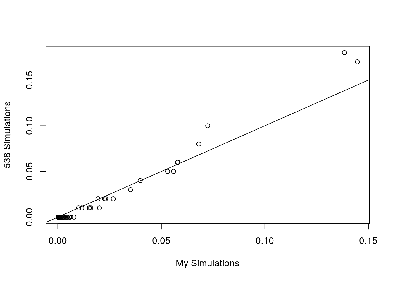
Our simulations are mostly comparable with the exception of the favorites that are a bit off.
I guess now is a good time to read 538’s How Our March Madness Predictions Work. So yeah, they calculate explicit probabilities that take into account matchups and teams' probabilities of advancing. But still… these are really far apart!
Looking at their very nice visualization of the bracket probabilities, it’s easy to see what goes wrong. Villanova has a 50% chance of advancing to the Final Four, whereas Virginia has only a 47% chance. That (and some earlier minor differences) are enough to swamp the 3% and 1% higher probabilities of winning the Final Four and National Championship games, respectively.
What to make of it? Maybe 538 would do well to actually run some simulations.? I think their conditional probabilities may be missing some interaction effects. Or maybe the interaction effects between teams really are that prominent. I don’t know.? Like I said, I don’t follow college sports :)
Edit 1:
After thinking about it overnight, 538’s probabilities are the probabilities of making it to a given round and winning. In order to simulate the tournament correctly, I need the probability of winning a game assuming they’ve made it to that round. To uncondition the variable like this I simply divide by the probability of making it to and winning the previous round. That’s the fifth line of code.
Edit 2:
Awkwardly, if you go and download 538’s data now, the numbers they published on Monday Forecast_date == 2018-03-12, were retroactively changed so that Virginia is now ranked second instead of first. I guess I’ll take that as a win.? (For the skeptics, here’s the video evidence.)
Above I implement Edit 1 using Monday’s original data. My analysis maintains that Villanova is favored, but brings the likelihood below 538’s projections. Villanova is still ranked first for me and second for them, as of the real Monday forecasts. And now Virginia’s Guard has broken his wrist, so everyone is jumping on the Villanova train regardless.
End of Edit
Finally, here are the most frequent results from the simulations:
t(t(apply(nat.champ.mat, 2, function(x){names(sort(table(x), decreasing = TRUE))[1]})))
##                         [,1]
## Midwest.First_Four1     "Syracuse"
## Midwest.First_Four2     "Pennsylvania"
## Midwest.First_Round1    "Kansas"
## Midwest.First_Round2    "Duke"
## Midwest.First_Round3    "Michigan State"
## Midwest.First_Round4    "Auburn"
## Midwest.First_Round5    "Clemson"
## Midwest.First_Round6    "Texas Christian"
## Midwest.First_Round7    "Rhode Island"
## Midwest.First_Round8    "Seton Hall"
## Midwest.Second_Round1   "Kansas"
## Midwest.Second_Round2   "Duke"
## Midwest.Second_Round3   "Michigan State"
## Midwest.Second_Round4   "Auburn"
## Midwest.Regional_Semis1 "Kansas"
## Midwest.Regional_Semis2 "Duke"
## Midwest.Regional_Final  "Kansas"
## East.First_Four1        "UCLA"
## East.First_Four2        "Radford"
## East.First_Round1       "Villanova"
## East.First_Round2       "Purdue"
## East.First_Round3       "Texas Tech"
## East.First_Round4       "Wichita State"
## East.First_Round5       "West Virginia"
## East.First_Round6       "Florida"
## East.First_Round7       "Butler"
## East.First_Round8       "Virginia Tech"
## East.Second_Round1      "Villanova"
## East.Second_Round2      "Purdue"
## East.Second_Round3      "Texas Tech"
## East.Second_Round4      "Wichita State"
## East.Regional_Semis1    "Villanova"
## East.Regional_Semis2    "Purdue"
## East.Regional_Final     "Villanova"
## West.First_Four1        "San Diego State"
## West.First_Four2        "Texas Southern"
## West.First_Round1       "Xavier"
## West.First_Round2       "North Carolina"
## West.First_Round3       "Michigan"
## West.First_Round4       "Gonzaga"
## West.First_Round5       "Ohio State"
## West.First_Round6       "Houston"
## West.First_Round7       "Texas A&M"
## West.First_Round8       "Florida State"
## West.Second_Round1      "Xavier"
## West.Second_Round2      "North Carolina"
## West.Second_Round3      "Michigan"
## West.Second_Round4      "Gonzaga"
## West.Regional_Semis1    "Gonzaga"
## West.Regional_Semis2    "North Carolina"
## West.Regional_Final     "North Carolina"
## South.First_Four1       "Loyola (IL)"
## South.First_Four2       "Maryland-Baltimore County"
## South.First_Round1      "Virginia"
## South.First_Round2      "Cincinnati"
## South.First_Round3      "Tennessee"
## South.First_Round4      "Arizona"
## South.First_Round5      "Kentucky"
## South.First_Round6      "Miami (FL)"
## South.First_Round7      "Texas"
## South.First_Round8      "Creighton"
## South.Second_Round1     "Virginia"
## South.Second_Round2     "Cincinnati"
## South.Second_Round3     "Tennessee"
## South.Second_Round4     "Arizona"
## South.Regional_Semis1   "Virginia"
## South.Regional_Semis2   "Cincinnati"
## South.Regional_Final    "Virginia"
## National_Semi1          "Villanova"
## National_Semi2          "Virginia"
## National_Champ          "Villanova"
Edit 3:
Regarding Edit 2, after some investigation 538’s estimates were changed to reflect that Virginia’s guard was injured. The problem is that when they changed their estimates on March 13th, their March 12th csv was presumably recompiled as well. This is a fantastic example of data governance issues and reproducibility that regulated industries have to take very seriously. 538 and March Madness? Not so much.